Use the old peak tracking algorithm in streaming data processing
The package also offers the infrastructure for the streaming data processing old way, where the peaks are tracked on each image in the series of the exposures and the peaks will be linked in the final. The crystal maps are generated by filling the peak intensity in the zero background.
Here, we show an example to process the streaming data. The streaming
data is obtained from the database and we will use databroker as the
interface to the database. In real use cases, the data will be from the
RunEngine.
Take a look at the raw data
First, we take a look at what our data is like. This is a grid scan on a crystal rod. At each pixel in the grid, there are multiple frames of diffraction images.
uid = UID["uid"][0]
run = DB[uid]
dask_array = run.xarray_dask()
dask_array.attrs = dict(run.start)
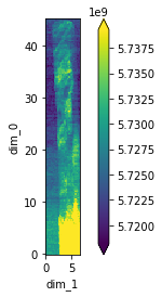
Here, we plot the spatial distribution of the total intensity. The upper part of the rod is made up by multiple crystalline domains while the lower part is full of powder.
stats1 = reshape(dask_array, "dexela_stats1_total")
plot_real_aspect(stats1);

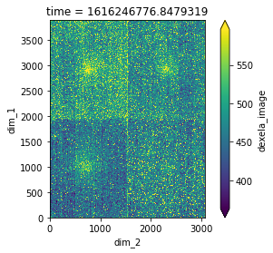
We select a image taken at the empty space. The image only contains dark current and air scattering. We will use this to subtract all other images in this scan.
image = dask_array["dexela_image"][4523].compute().mean(axis=0)
plot_real_aspect(image);

Use callbacks to process the event stream
Here, we use the callbacks to process the data in a stream. The frames
will be first go into the ImageProcessor. The frames will be
averaged and subtracted by the subtrahend. Because diffraction image
is non-negative, the negative pixels will be filled with zero. Then, the
results will be sent to PeakTracker. It will find the Bragg peaks on
the images and output each peak as a single event. The data will be
dumped to DB2. During this process, TrackLinker will monitor the
events. If all peaks have been found in all images, it will start
linking the peaks and output where the same Bragg peak is on a series of
images. The results will also be recorded in the database.
The argument dexela_image is the name of the data key of the data in
the event stream. diameter=15, percentile=80, separation=100 are the
key words for the trackpy.locate. search_range=50 is the key
word for the trackpy.link. Please see the documents of
trackpy for
more information.
Here, the BestEffortCallback is used to print out the status of
ImageProcessor. It is optional and does nothing to the data.
ip = ImageProcessor("dexela_image", subtrahend=image)
pt = PeakTracker("dexela_image", diameter=15, percentile=80, separation=100)
tl = TrackLinker(db=DB2, search_range=50)
bec = BestEffortCallback()
bec.disable_plots()
tl.subscribe(DB2.insert)
pt.subscribe(tl)
pt.subscribe(DB2.insert)
ip.subscribe(pt)
ip.subscribe(bec);
We pipe the data from our database to this callback function.
with Filler(
    handler_registry=dict(DB.reg.handler_reg),
    inplace=True,
    root_map=DB.reg.root_map
) as filler:
    for name, doc in run.documents(fill=False):
        filler(name, doc)
        ip(name, doc)
Use servers to process the real time event stream
We are basically replaying the data processing procedure in the last section. In this section, we will learn how the data is processed at the beamline in “real time”. We need to setup a server that wraps the callback function in last section. An example script is show here.
!cat server.py
import numpy as np
from databroker import Broker
from bluesky.callbacks.best_effort import BestEffortCallback
from crystalmapping.callbacks import ImageProcessor, PeakTrackor, TrackLinker
from bluesky.callbacks.zmq import RemoteDispatcher

# load the image to use
image = np.load("./data/PARAMID-2_background_1.npy", allow_pickle=True)

# create a remote dispatcher to receive the dispatch the data
rd = RemoteDispatcher(address=("localhost", 5568), prefix=b'raw')

# create the callback
ip = ImageProcessor("dexela_image", subtrahend=image)
pt = PeakTracker("dexela_image", diameter=15, percentile=80, separation=100)
tl = TrackLinker(db=DB2, search_range=50)
bec = BestEffortCallback()
bec.disable_plots()
tl.subscribe(DB2.insert)
pt.subscribe(tl)
pt.subscribe(DB2.insert)
ip.subscribe(pt)
ip.subscribe(bec)

# subscribe the callback to the dispatcher
rd.subscribe(ip)

# start the server
if __name__ == "__main__":
    print("Start the server ...")
    rd.start()
To start the server, we will run:
python server.py
Then, this server will receive the data from “localhost:5568” with prefix “raw” and process the data using the callback defined in the script.
Pipe the data into the database
We can also publish the data in the database to the server using
Publisher. Here, we show an example to publish our data to
“localhost:5567”. The server will process the data just like it is from
the beamline devices.
pub = Publisher("localhost", 5567)
with Filler(
    handler_registry=dict(DB.reg.handler_reg),
    inplace=True,
    root_map=DB.reg.root_map
) as filler:
    for name, doc in run.documents(fill=False):
        filler(name, doc)
        pub(name, doc)